Python and the 2D graphics lib Cairo
Introduction
Cairo is a 2D graphics library with support for multiple output devices. Currently supported output targets include the X Window System, Quartz, Win32, image buffers, PostScript, PDF, and SVG file output. Experimental backends include OpenGL, XCB, BeOS, OS/2, and DirectFB.
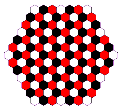
This little article will take the fast train of "quick and dirty" to show you how to draw something with the Cairo lib. As an example we will use a six players chess board with hexagonal tiles.
Geometry of hexagonal tiles
In the beginning we have to spend some thoughts on the geometry of hexagons and how to put them to their places in the easiest way.
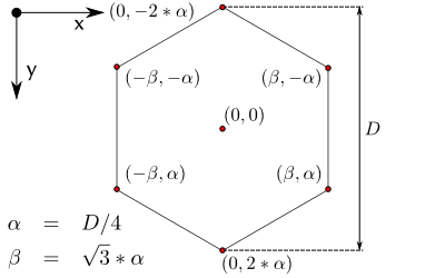
The above figure shows the geometric properties of a hexagon. The shown values are obtained using simple trigonometry. The figure even shows two import facts about the Cairo lib:
- The orientation of the cartesian system.
- By default the origin of the system is in the upper left corner of an image, but for trigonometry the origin was set in the middle of the hexagon.
Cairo's coordinate system
The cartesian coordinate system of the cairo module can be treated as known from mathematics. The Context class provides methods for coordinate transformations as indicated in the figure below.
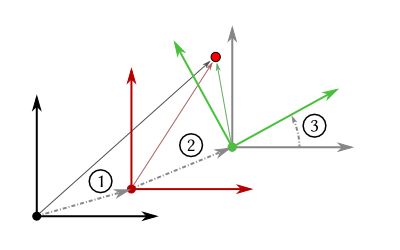
In the figure we can see the two most important coordinate transformations: translation (1 and 2) and rotation (3). The Context's coordinate system can be altered in any arbitrary way. Additionally some sort of stack is provided which remembers all transformations.
The save method of the Context remembers the current coordinate system and the restore method changes the coordinate system back to the last stored system. Thus one can easily undo a transformation.
In this example we will use this knowledge to write our script in an elegant way.
Philosophy of Cairo
The idea is similar to offset printing. In the end we want an image containing colored pattern, but to get there we have to do some steps:
- We have to define an image plane the so-called ImageSurface.
- We define the pattern in a so-called Context.
- Afterwards -- or prior to that -- we choose a color.
- Then we put the pattern to the surface. Therefore we can choose between printing the lines (stroke) or filling the pattern (fill).
- Finally we have to save the image to a file.
The module in action
Painting the canvas (rectangle)
First of all we need to define the surface for the image and a context. the ImageSurface class expects three arguments specifying color format, width and height (integer, in pixels).
surface = cairo.ImageSurface (cairo.FORMAT_ARGB32, width, height)
ctx = cairo.Context (surface)
If you would like to have a solid background color instead of a transparent background, you can fill the surface with a rectangle. Therefore you need a color, of course.
ctx.set_source_rgb(1,1,1)
ctx.rectangle(0,0,width,height)
ctx.fill()
As you can see above, we have chosen a RGB color space. In cairo one does not use the hexadecimal notation but the value range [0,1]. Once a source color is specified it is used until it is changed. So if we want to draw something else to the surface, we have to change the color therebefore. Otherwise we will still see only a white surface.
The rectangle has upper left corner coordinates, here (0,0), and an extent on the surface, here (width, height). Using the fill method the entire surface is painted white.
Drawing a structure (path)
Now that we have painted our background white we want to actually draw something more complicated. A hexagon is a slightly less basic structure and not provided by a method of the Context. Therefore we have to draw it ourselves using lines (aka path).
field_colors = ((1,1,1), (0,0,0), (1,0,0))
p = (
    (math.sqrt(3)*D/4., D/4.),
    (0, D/2.),
    (-math.sqrt(3)*D/4., D/4.),
    (-math.sqrt(3)*D/4., -D/4.),
    (0, -D/2.),
    (math.sqrt(3)*D/4.,-D/4.)
)

def hexagon(ctx,color):
    for pair in p:
        ctx.line_to(pair[0],pair[1])
    ctx.close_path()
    ctx.set_source_rgb(0,0,0)
    ctx.stroke_preserve()
    ctx.set_source_rgb(*field_colors[color%3])
    ctx.fill()
In p the coordinates of the edges of the hexagon are stored. The tuple field_colors holds three different RGB color values (white, black, red). Our function hexagon expects the Context instance and an integer in the variable color.
The function hexagon adds the coordinates of the six corners to the path by using the method line_to. So far we have a hexagon with one side open. To close it we simly call close_path or we add the coordinates of the first corner again. As you can see each hexagon will get a black contour. The method stroke_preserve paints the line and keeps the previous structure in the Context so that we can reuse it -- which we do by filling it with another color.
Filling the Surface with Heaxagons
Now that we have a function that draws nice hexagons, we can start to fill the entire surface with them. For our hexagonal chess board we want to have a defined number of fields on each side and no unneccessary white space, so we do some math to fit the chess board perfectly onto the surface:
D = 33
# diameter of hexagon in pixels
shift_x = (math.sqrt(3)*D/2., 0)
# vectorial distance to next hexagon in row
shift_y = (math.sqrt(3)*D/4., 3*D/4.)
# vectorial distance to hexagon in next row
side_fields = 7
# number of fields along each side
width = int((2*side_fields-1)*math.sqrt(3)*D/2.+3*D/4.)+1
# with of surface plus some border in pixels
height = int((2*side_fields-1)*3*D/4.+2*D)+1
# with of surface plus some border in pixels
Having all geometric information together we can now start to iterate through the chess board and draw hexagons:
fields_in_line = side_fields
increment, decreasing = 1, 0
ctx.translate((side_fields-1)*math.sqrt(3)*D/4.,D)
for j in range(2*side_fields-1):
	if fields_in_line > 2*side_fields-2:
		increment = -1
	for i in range(fields_in_line):
		ctx.translate(shift_x[0],shift_x[1])
		hexagon(ctx,i+j+decreasing)
	ctx.translate(-fields_in_line*shift_x[0],-fields_in_line*shift_x[1])
	ctx.translate(-increment*shift_y[0],shift_y[1])
	if increment == -1:
		decreasing += 1
	fields_in_line += increment
surface.write_to_png('hexach.png')
![]() First we translate to the center of the hexagon in the upper left corner of the chess board. Then we iterate through hexagons of a row by translating the coordinate system by shift_x. At the end of the row we have to get back to the first hexagon in the next row. Therefore we go back to the first hexagon's position in the current row and depending on whether the number of hexagons in the next row is in- or decresed we go the closest position left or right in the next row (see image on the left).
First we translate to the center of the hexagon in the upper left corner of the chess board. Then we iterate through hexagons of a row by translating the coordinate system by shift_x. At the end of the row we have to get back to the first hexagon in the next row. Therefore we go back to the first hexagon's position in the current row and depending on whether the number of hexagons in the next row is in- or decresed we go the closest position left or right in the next row (see image on the left).
In each row iteration we increase the number of hexagons by one until we reach the maximum number of hexagons per row. Then we decrease the number of hexagons per row by one.
Finally we save the image to the file hexach.png.
The result
This is the final image.