Solving a PDE

In this first example we want to solve the Laplace Equation (2) a special case of the Poisson Equation (1) for the absence of any charges.

(1)
(2)

Prior to actually solving the PDE we have to define a mesh (or grid), on which the equation shall be solved, and a couple of boundary conditions. Lines 6-9 define some support variables and a 2D mesh. Lines 10-12 define further support variables, which are used later to define boundary conditions and save the result in NumPy arrays.

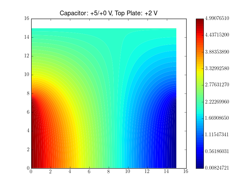
Lines 14-21 define the physical quantitiy (potential in the code, \phi in the above equaitons), the equation with this quantity, that needs to be solved, and the boundary conditions. In this example the boundary conditions represent three capacitor plates thus that the mesh shows the space between the plates. One plate is located at the top and extends along the entire x-range. The two other plates are at the left and right hand side, respectively, cover only the y<y0 range.

As shown in this example, boundary conditions (BCs) are objects of type FixedValue or FixedFlux (not shown). If more than one BC need to be defined, this can be done in a Python list or tuple. But notice: FiPy takes the term boundary condition very seriously. Boundary conditions can only be defined on so called exterior faces. Thus, if boundary conditions for a given problem cannot be applied onto the surfaces of a "common" mesh (line, square or cube), one has to construct a mesh suitable for the problem using a tool called gmsh [2].

Line 23 starts the actual PDE solving algorthm.

Lines 26-27 store the solution in a file. The specified file extensions determines the format of the output. Omitting arguments to viewer.plot() starts an interactive display module (e.g. Matplotlib, Mayavi2, etc.).

In case of "common" meshes it is rather easy to convert the CellVariable into a NumPy array as is shown in lines 31-39. In case of a uncommon mesh one would have to call the __call__() method of the CellVariable and evaluate each point for a given coordinate (will be shown in another example).

#!/usr/bin/env python

from fipy import *
import sys

nx = 300
dx = 0.05
L = nx * dx
mesh = Grid2D(dx=dx,dy=dx,nx=nx,ny=nx)
x,y = mesh.getCellCenters()
x0,y0 = L/2,L/2
X,Y = mesh.getFaceCenters()

potential = CellVariable(mesh=mesh, name='potential', value=0.)
potential.equation = (DiffusionTerm(coeff = 1.) == 0.)

bcs = (
    FixedValue(value=5,faces=mesh.getFacesLeft() & (Y<y0) ),
    FixedValue(value=0,faces=mesh.getFacesRight() & (Y<y0) ),
    FixedValue(value=2,faces=mesh.getFacesTop() ),
)

potential.equation.solve(var=potential, boundaryConditions=bcs)

# The default visualization method
viewer = viewers.Viewer(vars=(potential,))
viewer.plot("/path/to/output.vtk")

# The follow evaluation of the solution is only
# possible with "common" meshes.
result = pylab.array(potential)
result = result.reshape((nx,nx))
xx,yy = pylab.array(x), pylab.array(y)
xx,yy = xx.reshape((nx,nx)), yy.reshape((nx,nx))

pylab.title("Capacitor: +5/+0 V, Top Plate: +2 V")
pylab.contourf(xx,yy,result,levels=pylab.linspace(result.min(),result.max(),64))
pylab.colorbar()
pylab.show()

References

1. http://www.ctcms.nist.gov/fipy/
2. http://geuz.org/gmsh/
3. R. Pavelka, "Numerical solving of anisotropic elliptic equation
   on disconnected mesh using FiPy and Gmsh", 2012 (Mirror)
4. J. E. Guyer, D. Wheeler & J. A. Warren, "FiPy: Partial Differential Equations with Python", Computing in Science & Engineering 11(3) pp. 6—15 (2009)
5. C. Geuzaine and J.-F. Remacle. "Gmsh: a three-dimensional finite element mesh generator with built-in pre- and post-processing facilities". International Journal for Numerical Methods in Engineering, Volume 79, Issue 11, pages 1309-1331, 2009